Welcome to the Network Engineering Domain
Pape O. Fall's Blog
EIGRP stands for Enhanced Interior Gateway Routing Protocol which is just like the name implies, an enhanced version of the legacy IGRP. It is considered as an “Advanced Distance Vector Protocol” which uses 5 different type of packets to exchange information:
-Hello: Hello packets are used to discover EIGRP neighbors.
-Update: Updates are mainly used for route advertisement and they are only sent when a change occurs which makes this routing protocol a bit more attractive than others. It uses the multicast address 224.0.0.10.
-Ack: This packet type acknowledges the receipt of data.
-Query: This packet type is used to find an alternate path to a destination when all routes in the topology table have failed.
-Reply: This packet type is sent in response to query packets to instruct the originator not to recompute the route because feasible successors exist.
In this topic, I will explain the meaning of the different variables that play a major role in route computation. I will also show you how to alter the route selection so you can have full control in terms of where to forward your traffic. We will be using the following topology…

You can see here that we have different interface types. Hence, different interface bandwidth capacity. This will come in handy in a minute but before we hop onto the consoles, I would like to show you why I call EIGRP “Mr. Friendly”.
First and foremost, the initiator sends a hello packet to the multicast address 224.0.0.10 via TCP…
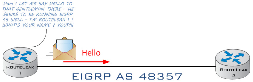
The receiver then responds with a “Hello”.
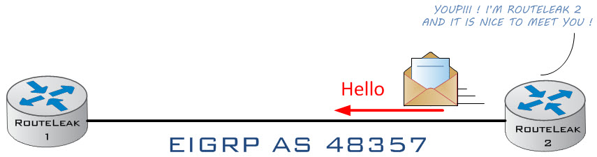
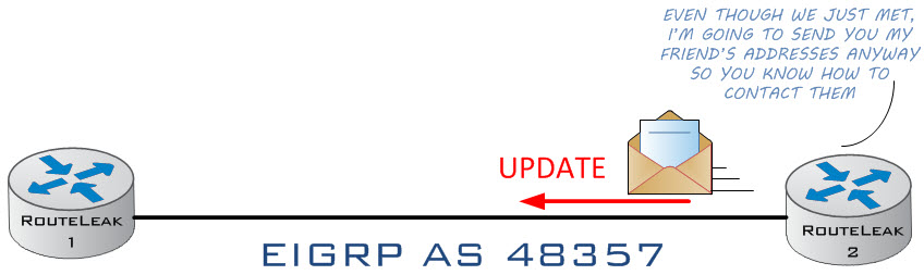
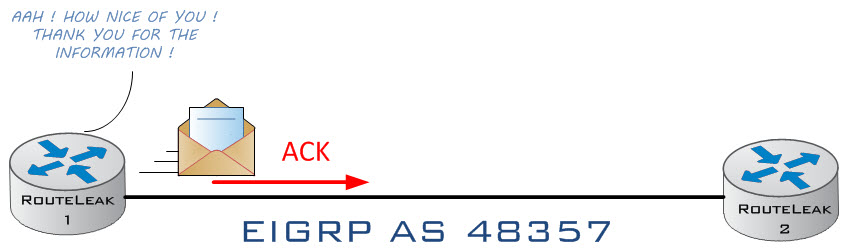
Right off the bat, the receiver offers to share its routing information.
The initiator then acknowledges the receipt of the information…
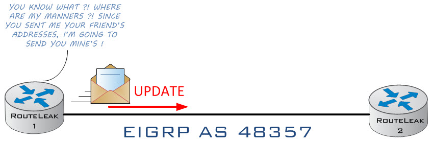
And of course as you may have already guessed, the initiator does the same…
The receiver acknowledges that the routes are received and we are now fully converged…
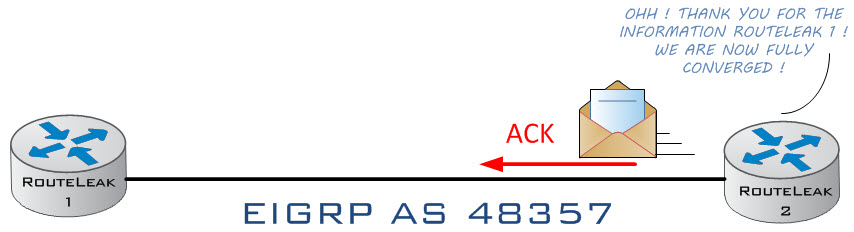
At this point, the neighbor relationship has been formed and both routers are fully converged. A couple of things to remember here are:
*In order to form an adjacency, the following conditions must be met first:
-Hello packets must make it across on both direction meaning the router must receive the hello packet and vice versa
-The EIGRP AS (Autonomous System) number must be the same. In our case, the AS number is 48357
-The K values must be identical on both side. I’ll touch on this in a sec
*Once adjacency is formed, EIGRP uses the following tables to store information:
-Neighbor Table: IP addresses of directly connected routers
-Topology Table: This is where all EIGRP learned routes are stored – We will see it when we hop onto the console
-Routing Table: This is where EIGRP best routes from other routing process are stored
Okay, let’s move on to some stuff that are much more exciting than this. How does EIGRP calculate the best path ??
Well by default, EIGRP uses the minimum bandwidth to a destination along with the ∑ delay to compute routing metrics. Note that various values are considered in the metric formula which are K1 through K5 but by default K1=K3=1 and K2=K4=K5=0. Below are the K values and the formula used to compute routes (The formula has been simplified since K2, K4 and K5 are equal to Zero)…

Note that the K values on one router needs to be identical to the K values of the peer router in order to establish adjacency.
All right ! Now that we know about the K values and the metric formula, let’s talk a bit about certain key terms that are extremely useful when dealing with EIGRP.
One of the advantage of EIGRP is its capability to compute a backup route and leverage its fast convergence feature to provide redundancy in case the primary route fails. The primary route is called the “Successor” and the backup route is called the “Feasible Successor”. Let’s talk about the definition of the some of the key terms. Again, these are the key components that would allow you to manipulate your inbound/outbound traffic. It is important to be familiar with them especially when working in an environment running EIGRP.
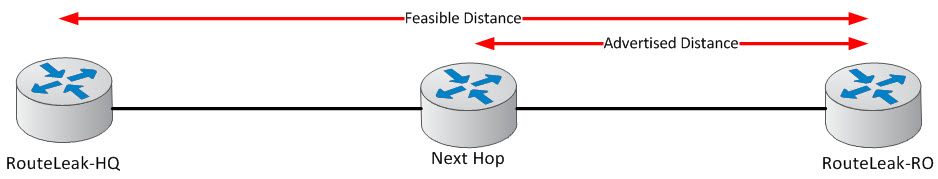
Advertised distance (AD): The metric (Cost) advertised by the next hop neighbor to reach the destination
Feasible distance (FD): Cost to reach the next hop router + AD (Advertised Distance)
Successor: The primary route (Best route) to reach a destination. The successor route is installed in the routing table
Feasible successor: The backup route (2nd best route). Note that in order to become a “Feasible Successor”, the path must have a reported distance or advertised distance that is less than the FD of the current successor. I’ll show you what it means once we get into the consoles.
Let’s get a visual of what we’ve just discussed…
Ok very nice ! Let’s now hop onto the consoles and I’ll show you the above in action. So, we will use the first topology in this post. Let’s configure all interface IP addresses as well as EIGRP 48357 on all routers. Note that our goal is to see what path EIGRP prefers to get to the loopback addresses from either the HeadQuarter or the Remote Office. Once we determine that, we will then manipulate the route so traffic can flow outbound from either site via a different path. I’ll show you different methods that can be used and we will see everything we’ve learned so far in action…
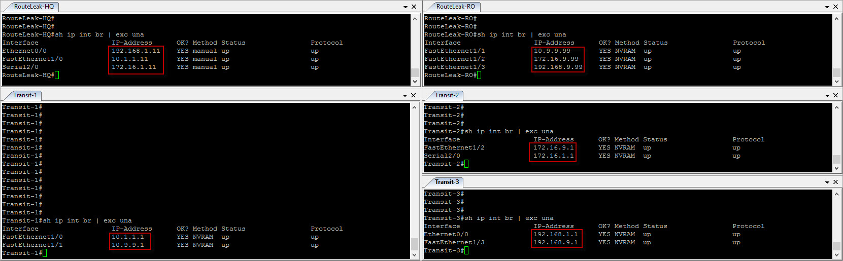
All right ! We’ve done with our IP addresses configuration, let’s now configure EIGRP process 48357. The steps are very straight forward; First we need to enable EIGRP process with an arbitrary AS number (AS number can vary from 1 to 65535) by using the command “router eigrp 48357”. Then we will need to use the “network” command in order to advertise the adequate prefixes in EIGRP. Let’s do that…
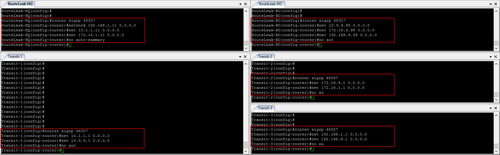
That’s all there is to it ! There is another EIGRP mode called “EIGRP named mode” which allows you to define all related EIGRP configuration under the EIGRP process itself… For instance, if you were to configure Authentication with the mode that we are using right now, we would have to do it at the interface level… But with EIGRP named mode, you can do it under the process by referencing the af-interface… You can also call out different address families under the same process but we can see that some other time in a different post.
Okay, as of right now… We have EIGRP configured on all routers. Typically, you’d see a console message letting you know that an adjacency has been formed (Since we are consoled in) but I purposely disabled logging console for the sake of this example. Let’s now verify and make sure we have adjacency…
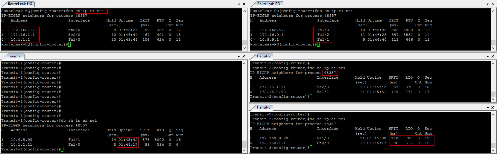
Ahh ! Fantastic ! Here we can see that we in fact have established adjacency across our network. If you refer to the topology above, you can see the neighbor IP addresses we are peering with on each router. Let’s analyze the output here…
So, we’ve ran the command “show ip eigrp neighbor” which provide us with the EIGRP neighbor table from each router. Here we can the neighbor IP addresses we are peering with – We can also see the interfaces we are learning those routes from – Our autonomous system is also part of the output which is 48357 – The “Uptime” is the amount of time we’ve maintained the adjacency – The “SRTT” is the amount of time in ms it takes to send a EIGRP packet and receive an acknowledgment back – The “RTO” is the holdown time before EIGRP retransmit a packet – The “Q” means the number of EIGRP packets in the queue waiting to be released – The “Seq Num” is the sequence number of the last update.
Let’s configure our loopback addresses and advertise them via EIGRP. Let’s then check if we routes to either loopback from both sides…
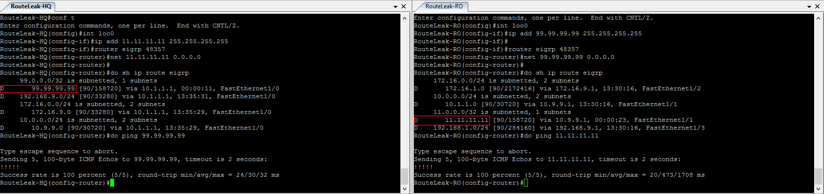
All right ! All set ! We can clearly see here that the HQ is learning the RO looback address via EIGRP and vice versa. The “D” in front of the IP address tells us that the prefix is being learned via EIGRP.
Remember the “K” values we’ve talked about earlier ? Let me show you how to get them…
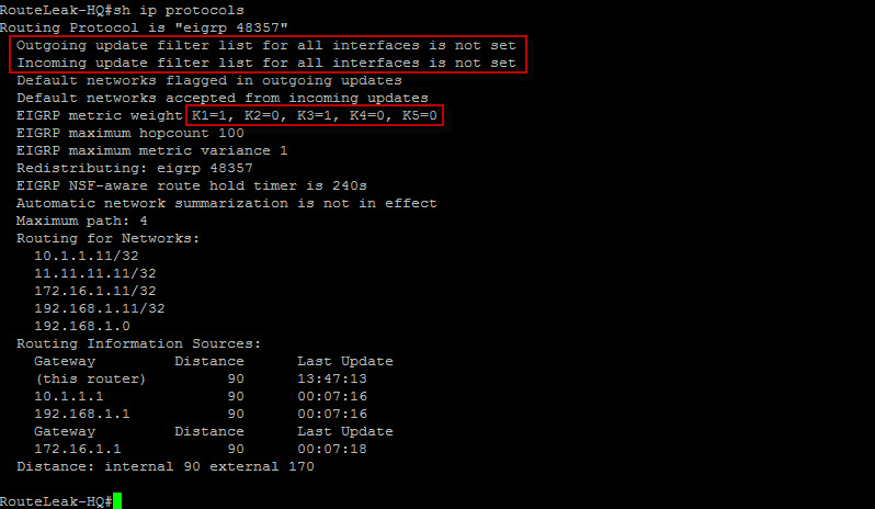
The output of the “show ip protocols” displays great amount of information. I personally likes this command because it reveals not only the “K” values but any filtering mechanism that might be blocking your traffic (This will come in handy in the Troubleshooting section).
Let’s now find out how the HQ is getting to the RO loopback address and then alter that…
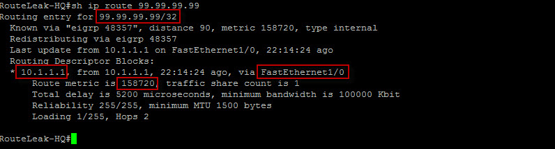
Here we can see that RouteLeak-HQ is prefering the path through Transit 1 via interface Fa1/0. The next hop address is 10.1.1.1 and the route metric is 158720 (Feasible Distance). This all makes perfect sense because EIGRP is preferring the faster link over the others. Let’s check the topology table and see what we have…
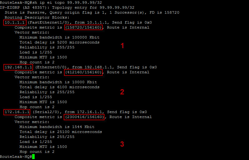
All right, the primary path is denominated “1” here and it is in fact the one installed in the main routing table. If we look at the 2nd option, we can clearly see here that the feasible distance of the path through eth0/0 is higher than the one of the primary; Hence, making it less desirable (412160 > 158720). The same analogy applies for the 3rd option.
It is important to note that both the 2nd and 3rd options meet the feasible successor condition which states that the AD must be less than the FD of the successor. In our case, 156160 < 158720.
Let me show you how to use the variance command to manipulate the traffic conducive to forward data over multiple paths. So, the formula involving the variance command is as followed:
FD (of the FS) = FD (of the S) * Variance – Basically in order to get the FD of the Feasible Successor, we will need to multiply the FD of the Successor by an integer and that decimal number is the variance.
Based on the equation above, we can quickly determine the variance by computing basic math – The formula will be as such:
FD (of the FS) / FD (of the S) = Variance
All right ! in our case we have the following (Let’s use the path through Eth0/0 for now):
FD (of the FS) = 412160
FD (of the S) = 158720
Variance would be then equal to 412160/158720=2.596. Let’s round it up to 3 and configure it under the EIGRP process !
![]()
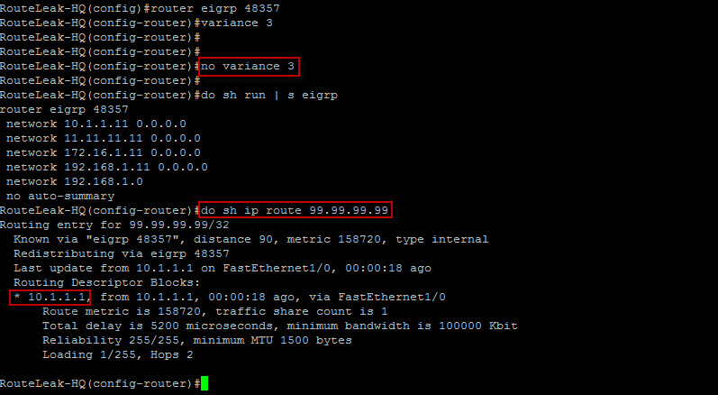
Let’s now check our routing table again…
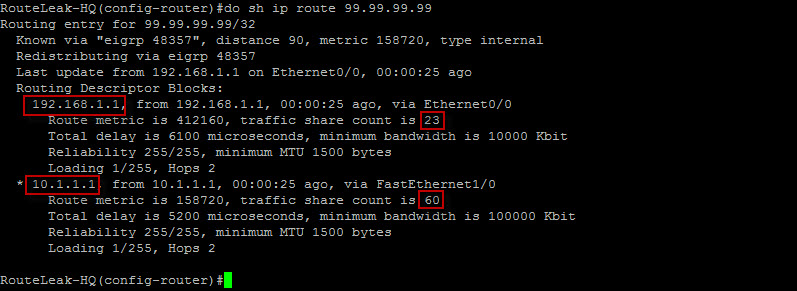
Look at this ! Now we have 2 transit paths to reach the loopback at the remote office in our main routing table ! This is called “Unequal Cost Load Balancing”. However, I do not agree with the term but that’s my personal opinion 😉 To me, whenever the word “Balance” is used, it basically means that the cumulative load is split in an equal format and dispersed via different paths. In our case here, we are not sharing the load equally between the Fastethernet and Ethernet links… You can see the share count on the Fastethernet here is 60 whereas the one on the Ethernet is 23.
To me, it should be called “Load Sharing”. It’s clear to me that we are sharing the load between these 2 paths whether they are equal or not. “Sharing” does not mandate equal quantum but “Balancing” does. That’s just my 2 cents but let’s move on.
Let’s now remove the variance command. I would like to show you how the EIGRP metric formula is used to calculate the FD. I will then show you how to leverage the formula to load balance traffic via transit 1 and transit 3 for instance.
The variance command has been removed and we now only have a single path to reach the loopback address. Let’s check the topology table again and use the metric formula to load balance the traffic…
Before we load balance the traffic, let’s test the formula and see if we get 158720 (Primary path).
Our metric formula is as followed: Metric = 256*[(10^7 / min. BW) + ∑Delay)]
So, take a look section 1 in the output above. Can you see that the minimum bandwidth is “100000” and the total delay is “5200” ? Let’s now calculate the metric. So we have so far:
Minimum Bandwidth = 100000 Kbit
∑ Delay = 5200 microseconds
So, metric = 256*[(10^7 / 100000) + 520)]. Noticed how in the formula, we have 520 instead of 5200 ? Well, that’s because when computing we have to use the delay in tens of microseconds so we have to devide the delay metric (in microseconds) by 10.
All right, so that gives us: metric = 256*[(100) + 520)] which then gives us: metric = 256*(620) which results in metric = 158720
Very good ! We can clearly see that we have the same metric from the output.
Great ! Now, our goal is to load balance traffic between Transit 1 and Transit 3. You probably already guessed that to make it happen, both Feasible Distance will need to be the same from the HeadQuarter perspective which would lead us to have “412160” as a metric for both paths through Fa1/0 and Eth0/0.
All right, so from section 1 in the above picture, we have:
Minimum Bandwidth = 100000
∑ Delay = 5200
We need the metric to be = 412160
Humm ! To achieve the above metric, one value will need to be changed. Let’s change the minimum bandwidth value so we can get 412160 as a metric. We will be using basic math for this process.
412160 = 256*[(10^7 / bw)+ 520)]
Let’s minimize the equation by doing the following: 412160 / 256 = (10^7 / bw)+ 520)
So we now have: 1610 = (10^7 / bw)+ 520)
All right ! Let’s minimize the equation by doing the following: 1610 – 520 = 10^7 / bw
So now we have: 1090 = 10^7 / bw
Good ! Let’s minimize the equation by doing the following: bw = 10^7 / 1090
So now we have: bw = 9174.3119266055045871559633027523
Let’s go ahead and configure the bandwidth value (9174) under the Fa0/1 interface and check our routing and topology table…
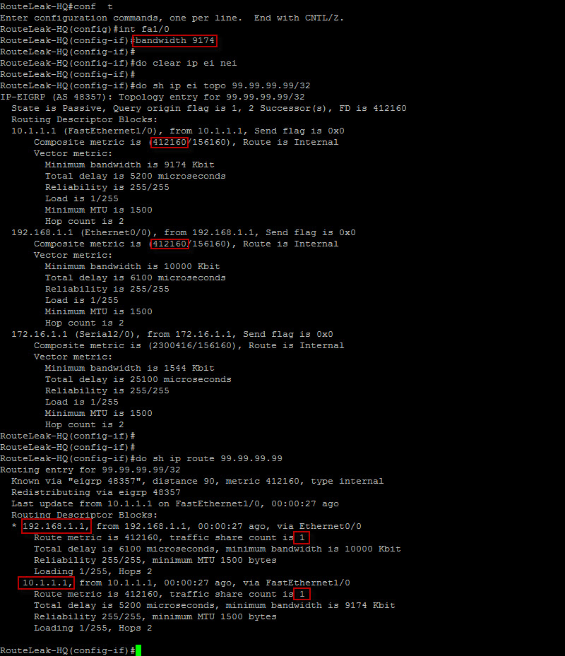
Ahh ! We have now achieved true load balancing between the 2 transit paths. We can clearly see here that both FD are identical (412160) now and we have both routes installed in our main routing table. This is a long one but I’m glad we got through it together !
Quick Tips: Note that changing the delay parameters might be your best option depending on the landscape of your network. The delay parameter is propagated downtream to all the routers giving you then a certain level of flexibility.
EIGRP Administrative Distance (Internal): 90
EIGRP Administrative Distance (External): 170
All right, it was a long one but there is much more to cover – We will see those in the troubleshooting section. I’ll talk to you guys later.
 Hello I'm Pape. My friends call me Pop. I'm CCIE #48357. I enjoy my field and love to share it with others. I love to write so I'm sharing my blog with you.
| M | T | W | T | F | S | S |
|---|---|---|---|---|---|---|
| 1 | ||||||
| 2 | 3 | 4 | 5 | 6 | 7 | 8 |
| 9 | 10 | 11 | 12 | 13 | 14 | 15 |
| 16 | 17 | 18 | 19 | 20 | 21 | 22 |
| 23 | 24 | 25 | 26 | 27 | 28 | 29 |
| 30 | ||||||
i learn a lot of material in your courses it help me a lot….. good continuation brother…
I’m glad it does ! Let me know if you have any questions…
Very helpfull blog bro ! thanks !
Thank you brother ! Haven’t written articles in a long time due to time constraint but will do soon
Thanks POP for the wonderful post. I am also looking the new BGP attribute in your post. DO you have any thing on the AIGP-BGP Accumulative IGP. I just looked an article in the below mentioned link, I am not sure about the same. Can you please help me to put some light on this
http://www.routexp.com/2017/11/bgp-attribute-aigp-bgp-accumulative-igp.html
Hello Singh,
I’ll work on writing an article with regards to this. In the meantime, you can check out my BGP article.
http://routeleak.com/bgp-border-gateway-protocol/